A guide to measuring long-term inequality in the exposure to crime at micro-area levels using 'Akmedoids' package

Authors:
Adepeju, M., Langton, S., and Bannister, J.
Big Data Centre, Manchester Metropolitan University, Manchester, M15 6BH

Date:
2021-08-25

Abstract

The 'akmedoids' package advances a set of R-functions for longitudinal clustering of long-term trajectories and determines the optimal solution based on the Caliński-Harabasz criterion (Caliński and Harabasz 1974). The package also includes a set of functions for addressing common data issues, such as missing entries and outliers, prior to conducting advance longitudinal data analysis. One of the key objectives of this package is to facilitate easy replication of a recent paper which examined small area inequality in the crime drop (see Adepeju et al. 2021). This document is created to provide a guide towards accomplishing this objective. Many of the functions provided in the akmedoids package may be applied to longitudinal data in general.

Introduction

Longitudinal clustering analysis is ubiquitous in social and behavioral sciences for investigating the developmental processes of a phenomenon over time. Examples of the commonly used techniques in these areas include group-based trajectory modeling (GBTM) and the non-parametric kmeans method. Whilst kmeans has a number of benefits over GBTM, such as more relaxed statistical assumptions, generic implementations render it more sensitive to outliers and short-term fluctuations, which minimises its ability to identify long-term linear trends in data. In crime and place research, for example, the identification of such long-term linear trends may help to develop some theoretical understanding of criminal victimization within a geographical space (Weisburd et al. 2004; Griffith and Chavez 2004). In order to address this sensitivity problem, we advance a novel technique named anchored kmedoids ('akmedoids') which implements three key modifications to the existing longitudinal kmeans approach. First, it approximates trajectories using ordinary least square regression (OLS) and second, anchors the initialisation process with median observations. It then deploys the medoids observations as new anchors for each iteration of the expectation-maximization procedure (Celeux and Govaert 1992). These modifications ensure that the impacts of short-term fluctuations and outliers are minimized. By linking the final groupings back to the original trajectories, a clearer delineation of the long-term linear trends of trajectories are obtained.

We facilitate the easy use of akmedoids through an open-source package using R. We encourage the use of the package outside of criminology, should it be appropriate. Before outlining the main clustering functions, we demonstrate the use of a few data manipulation functions that assist in data preparation. The worked demonstration uses a small example dataset which should allow users to get a clear understanding of the operation of each function.

Table 1. Data manipulation functions

SN	Function	Title	Description
1	data_imputation	Data imputation for longitudinal data	Calculates any missing entries (NA, Inf, null) in a longitudinal data, according to a specified method
2	rates	Conversion of ‘counts’ to ‘rates’	Calculates rates from observed ‘counts’ and its associated denominator data
3	props	Conversion of ‘counts’ (or ‘rates’) to ‘Proportion’	Converts ‘counts’ or ‘rates’ observation to ‘proportion’
4	outlier_detect	Outlier detection and replacement	Identifies outlier observations in the data, and replace or remove them
5	w_spaces	Whitespace removal	Removes all the leading and trailing whitespaces in a longitudinal data
6	remove_rows_n	Incomplete rows removal	Removes rows which contain ‘NA’ and ‘inf’ entries

1. Data manipulation

Table 1 shows the main data manipulation functions and their descriptions. These functions help to address common data issues prior to analysis, as well as basic data manipulation tasks such as converting longitudinal data from count to proportion measures (as per the crime inequality paper where akmedoids was first implemented). In order to demonstrate the utility of these functions, we provide a simulated dataset traj which can be called by typing traj in R console after loading the akmedoids library.

(i) "data_imputation" function

Calculates any missing entries in a data, according to a chosen method. This function recognizes three kinds of data entries as missing. These are NA, Inf, null, and an option of whether or not to consider 0’s as missing values. The function provides a replacement option for the missing entries using two methods. First, an arithmetic method which uses the mean, minimum or maximum value of the corresponding rows or columns of the missing values. Second, a regression method which uses OLS regression lines to estimate the missing values. Using the regression method, only the missing data points derive values from the regression line while the remaining (observed) data points retain their original values. The function terminates if there is any trajectory with only one observation in it. Using the 'traj' dataset, we demonstrate how the 'regression' method estimates missing values.

#installing the `akmedoids` packages
install.packages("devtools")
devtools::install_github("manalytics/akmedoids")

#loading the package
library(akmedoids)

#import and preview the first 6 rows of 'traj' object
data(traj)

head(traj)
#>   location_ids X2001 X2002 X2003 X2004 X2005 X2006 X2007 X2008 X2009
#> 1    E01012628     3     0     1     2     1     0     1     4     0
#> 2    E01004768     9    NA     2     4     7     5     1     3     1
#> 3    E01004803     4     3     0    10     2     3     6     6     8
#> 4    E01004804     7     3     9     3     2    NA     6     3     2
#> 5    E01004807     2   Inf     5     5     6    NA     3     5     4
#> 6    E01004808     8     5     8     4     1     5     6     1     1

#no. of rows
nrow(traj) 
#> [1] 10

#no. of columns
ncol(traj) 
#> [1] 10

The first column of the traj object is the id (unique) field. In many applications, it is necessary to preserve the id column in order to allow linking of outputs to other external datasets, such as spatial location data. Most of the functions of the akmedoids provides an option to recognise the first column of an input dataset as the unique field. The data_imputation function can be used to imput the missing data point of traj object as follows:

imp_traj <- data_imputation(traj, id_field = TRUE, method = 2, 
               replace_with = 1, fill_zeros = FALSE)
#> [1] "8 entries were found/filled!"

imp_traj <- imp_traj$CompleteData
#viewing the first 6 rows
head(imp_traj)
#>   location_ids X2001 X2002 X2003 X2004 X2005 X2006 X2007 X2008 X2009
#> 1    E01012628     3  0.00     1     2     1  0.00     1     4     0
#> 2    E01004768     9  6.44     2     4     7  5.00     1     3     1
#> 3    E01004803     4  3.00     0    10     2  3.00     6     6     8
#> 4    E01004804     7  3.00     9     3     2  3.90     6     3     2
#> 5    E01004807     2  3.92     5     5     6  4.36     3     5     4
#> 6    E01004808     8  5.00     8     4     1  5.00     6     1     1

The argument method = 2 refers to the regression technique, while the argument replace_with = 1 refers to the linear option (currently the only available option). Figure 1 is a graphical illustration of how this method approximates the missing values of the traj object.

Estimating the population data using the 'data_imputation' function

Obtaining the denominator information (e.g. population estimates to normalize counts) of local areas within a city for non-census years is problematic in longitudinal studies. This challenge poses a significant drawback to the accurate estimation of various measures, such as crime rates and population-at-risk of an infectious disease. Assuming a limited amount of denominator information is available, an alternative way of obtaining the missing data points is to interpolate and/or extrapolate the missing population information using the available data points. The data_imputation function can be used to perform this task.

The key step towards using the function for this purpose is to create a matrix, containing both the available fields and the missing fields arranged in their appropriate order. All the entries of the missing fields can be filled with either NA or null. Below is a demonstration of this task with a sample population dataset with only two available data fields. The corresponding input matrix is constructed as shown.

#import population data
data(popl)

#preview the data
head(popl)
#>   location_id census_2003 census_2007
#> 1   E01004809         300         200
#> 2   E01004807         550         450
#> 3   E01004788         150         250
#> 4   E01012628         100         100
#> 5   E01004805         400         350
#> 6   E01004790         750         850

nrow(popl) #no. of rows
#> [1] 11

ncol(popl) #no. of columns
#> [1] 3

The corresponding input dataset is prepared as follows and saved as population2:

#>   location_ids X2001 X2002 X2003 X2004 X2005 X2006 X2007 X2008 X2009
#> 1    E01004809    NA    NA   300    NA    NA    NA   200    NA    NA
#> 2    E01004807    NA    NA   550    NA    NA    NA   450    NA    NA
#> 3    E01004788    NA    NA   150    NA    NA    NA   250    NA    NA
#> 4    E01012628    NA    NA   100    NA    NA    NA   100    NA    NA
#> 5    E01004805    NA    NA   400    NA    NA    NA   350    NA    NA
#> 6    E01004790    NA    NA   750    NA    NA    NA   850    NA    NA

The missing values are estimated as follows using the regression method of the data_imputation function:

pop_imp_result <- data_imputation(population2, id_field = TRUE, method = 2, 
               replace_with = 1, fill_zeros = FALSE)
#> [1] "77 entries were found/filled!"

pop_imp_result <- pop_imp_result$CompleteData

#viewing the first 6 rows
head(pop_imp_result)
#>   location_ids X2001 X2002 X2003 X2004 X2005 X2006 X2007 X2008 X2009
#> 1    E01004809   350   325   300   275   250   225   200   175   150
#> 2    E01004807   600   575   550   525   500   475   450   425   400
#> 3    E01004788   100   125   150   175   200   225   250   275   300
#> 4    E01012628   100   100   100   100   100   100   100   100   100
#> 5    E01004805   425 412.5   400 387.5   375 362.5   350 337.5   325
#> 6    E01004790   700   725   750   775   800   825   850   875   900

Given that there are only two data points in each row, the regression method will simply generate the missing values by fitting a straight line to the available data points. The higher the number of available data points in any trajectory the better the estimation of the missing points. Figure 1 illustrates this estimation process.

(ii) "rates" function

Given a longitudinal data (\(m\times n\)) and its associated denominator data (\(s\times n\)), the 'rates' function converts the longitudinal data to ‘rates’ measures (e.g. counts per 100 residents). Both the longitudinal and the denominator data may contain different number of rows, but need to have the same number of columns, and must include the id (unique) field as their first column. The rows do not have to be sorted in any particular order. The rate measures (i.e. the output) will contain only rows whose id's match from both datasets. We demonstrate the utility of this function using the imp_traj object (above) and the estimated population data (‘pop_imp_result’).

#example of estimation of 'crimes per 200 residents'
crime_per_200_people <- rates(imp_traj, denomin=pop_imp_result, id_field=TRUE, 
                              multiplier = 200)

#view the full output
crime_per_200_people <- crime_per_200_people$rates_estimates

#check the number of rows
nrow(crime_per_200_people)
#> [1] 9

From the output, it can be observed that the number of rows of the output data is 9. This implies that only 9 location_ids match between the two datasets. The unmatched ids are ignored. Note: the calculation of rates often returns outputs with some of the cell entries having Inf and NA values, due to calculation errors and character values in the data. We therefore recommend that users re-run the data_imputation function after generating rates measures, especially for a large data matrix.

(iii) "props" function

Given a longitudinal data, the props function converts each data point (i.e. entry in each cell) to the proportion of the sum of their corresponding column. Using the crime_per_200_people estimated above, we can derive the proportion of crime per 200 people for each entry as follows:

#Proportions of crimes per 200 residents
prop_crime_per200_people <- props(crime_per_200_people, id_field = TRUE, scale = 1, digits=2)

#view the full output
prop_crime_per200_people
#>   location_ids X2001 X2002 X2003 X2004 X2005 X2006 X2007 X2008 X2009
#> 1    E01012628  0.10  0.13  0.04  0.09  0.21  0.19  0.05  0.14  0.17
#> 2    E01004768  0.12  0.28  0.13  0.09  0.09  0.17  0.04  0.08  0.00
#> 3    E01004803  0.08  0.11  0.16  0.13  0.17  0.16  0.17  0.15  0.17
#> 4    E01004804  0.07  0.07  0.00  0.18  0.04  0.06  0.12  0.08  0.24
#> 5    E01004807  0.15  0.08  0.18  0.06  0.04  0.08  0.12  0.04  0.06
#> 6    E01004808  0.11  0.11  0.18  0.14  0.22  0.11  0.16  0.13  0.16
#> 7    E01004788  0.02  0.06  0.06  0.07  0.11  0.09  0.07  0.08  0.17
#> 8    E01004790  0.18  0.16  0.19  0.09  0.03  0.13  0.16  0.02  0.04
#> 9    E01004805  0.17  0.00  0.07  0.15  0.09  0.00  0.10  0.28  0.00


#A quick check that sum of each column of proportion measures adds up to 1.  
colSums(prop_crime_per200_people[,2:ncol(prop_crime_per200_people)])
#> X2001 X2002 X2003 X2004 X2005 X2006 X2007 X2008 X2009 
#>  1.00  1.00  1.01  1.00  1.00  0.99  0.99  1.00  1.01

In line with the demonstration in Adepeju et al. (2021), we will use these proportion measures to demonstrate the main clustering function of this package.

(iv) "outlier_detect" function

This function is aimed at allowing users to identify any outlier observations in their longitudinal data, and replace or remove them accordingly. The first step towards identifying outliers in any data is to visualize the data. A user can then decide a cut-off value for isolating the outliers. The outlier_detect function provides two options for doing this: (i) a quantile method, which isolates any observations with values higher than a specified quantile of the data values distribution, and (ii) a manual method, in which a user specifies the cut-off value. The ‘replace_with’ argument is used to determine whether an outlier value should be replaced with the mean value of the row or the mean value of the column in which the outlier is located. The user also has the option to simply remove the trajectory that contains an outlier value. In deciding whether a trajectory contains outlier or not, the count argument allows the user to set an horizontal threshold (i.e. number of outlier values that must occur in a trajectory) in order for the trajectory to be considered as having outlier observations. Below, we demonstrate the utility of the outlier_detect function using the imp_traj data above.

(v) "w_spaces" function

Given a matrix suspected to contain whitespaces, this function removes all the whitespaces and returns a cleaned data. ’Whitespaces’ are white characters often introduced during data entry, for instance by wrongly pressing the spacebar. For example, neither " A" nor “A” equates “A” because of the whitespaces that exist in them. They can also result from systematic errors in data recording devices.

(vi) "remove_rows_n" function

This function removes any rows in which an ‘NA’ or an ‘Inf’ entry is found.

#Plotting the data using ggplot library
library(ggplot2)
#> Warning: package 'ggplot2' was built under R version 4.0.5
#library(reshape2)

#converting the wide data format into stacked format for plotting
#doing it manually instead of using 'melt' function from 'reshape2'

#imp_traj_long <- melt(imp_traj, id="location_ids") 

coln <- colnames(imp_traj)[2:length(colnames(imp_traj))]
code_ <- rep(imp_traj$location_ids, ncol(imp_traj)-1)
d_bind <- NULL
  for(v in seq_len(ncol(imp_traj)-1)){
    d_bind <- c(d_bind, as.numeric(imp_traj[,(v+1)]))
  }

code <- data.frame(location_ids=as.character(code_))
variable <- data.frame(variable=as.character(rep(coln,
                        each=length(imp_traj$location_ids))))
value=data.frame(value = as.numeric(d_bind))

imp_traj_long <- bind_cols(code, variable,value) 
  
#view the first 6 rows
head(imp_traj_long)
#>   location_ids variable value
#> 1    E01012628    X2001     3
#> 2    E01004768    X2001     9
#> 3    E01004803    X2001     4
#> 4    E01004804    X2001     7
#> 5    E01004807    X2001     2
#> 6    E01004808    X2001     8

#plot function
p <-  ggplot(imp_traj_long, aes(x=variable, y=value,
            group=location_ids, color=location_ids)) + 
            geom_point() + 
            geom_line()

#options(rgl.useNULL = TRUE)
print(p)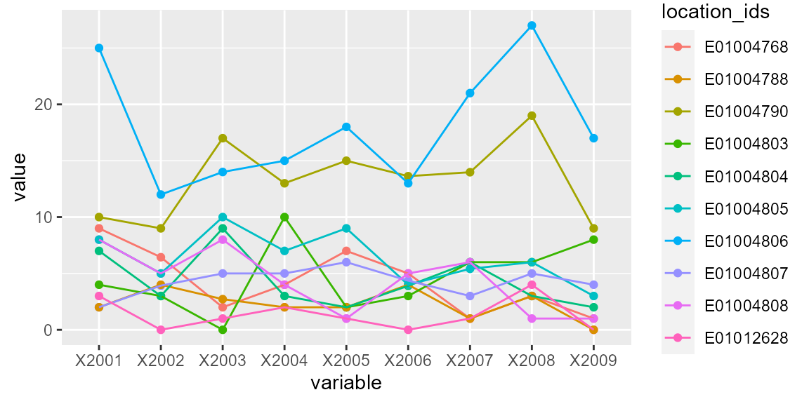

Figure 2: Identifying outliers

Figure 2 is the output of the above plot function.

Based on Figure 2 if we assume that observations of x2001, x2007 and x2008 of trajectory id E01004806 are outliers, we can set the threshold argument as 20. In this case, setting count=1 will suffice as the trajectory is clearly separable from the rest of the trajectories.

imp_traj_New <- outlier_detect(imp_traj, id_field = TRUE, method = 2, 
                              threshold = 20, count = 1, replace_with = 2)
#> [1] "1 trajectories were found to contain outlier observations and replaced accordingly!"
#> [1] "Summary:"
#> [1] "*--Outlier observation(s) was found in trajectory 10 --*"

imp_traj_New <- imp_traj_New$Outliers_Replaced 

#options(rgl.useNULL = TRUE)
print(imp_traj_New)
#>    location_ids X2001 X2002 X2003 X2004 X2005 X2006 X2007 X2008 X2009
#> 1     E01012628  3.00  0.00  1.00     2     1  0.00  1.00  4.00     0
#> 2     E01004768  9.00  6.44  2.00     4     7  5.00  1.00  3.00     1
#> 3     E01004803  4.00  3.00  0.00    10     2  3.00  6.00  6.00     8
#> 4     E01004804  7.00  3.00  9.00     3     2  3.90  6.00  3.00     2
#> 5     E01004807  2.00  3.92  5.00     5     6  4.36  3.00  5.00     4
#> 6     E01004808  8.00  5.00  8.00     4     1  5.00  6.00  1.00     1
#> 7     E01004788  2.00  4.00  2.72     2     2  4.00  1.00  3.00     0
#> 8     E01004790 10.00  9.00 17.00    13    15 13.63 13.98 19.00     9
#> 9     E01004805  8.00  5.00 10.00     7     9  4.00  5.41  6.00     3
#> 10    E01004806 14.83 12.00 14.00    15    18 13.00 14.83 14.83    17

#imp_traj_New_long <- melt(imp_traj_New, id="location_ids") 

coln <- colnames(imp_traj_New)[2:length(colnames(imp_traj_New))]
code_ <- rep(imp_traj_New$location_ids, ncol(imp_traj_New)-1)

d_bind <- NULL
  for(v in seq_len(ncol(imp_traj_New)-1)){
    d_bind <- c(d_bind, as.numeric(imp_traj_New[,(v+1)]))
  }

code <- data.frame(location_ids=as.character(code_))
variable <- data.frame(variable=as.character(rep(coln,
              each=length(imp_traj_New$location_ids))))
value=data.frame(value = as.numeric(d_bind))

imp_traj_New_long <- bind_cols(code, variable,value)

#plot function
#options(rgl.useNULL = TRUE)
p <-  ggplot(imp_traj_New_long, aes(x=variable, y=value,
            group=location_ids, color=location_ids)) + 
            geom_point() + 
            geom_line()

#options(rgl.useNULL = TRUE)
print(p)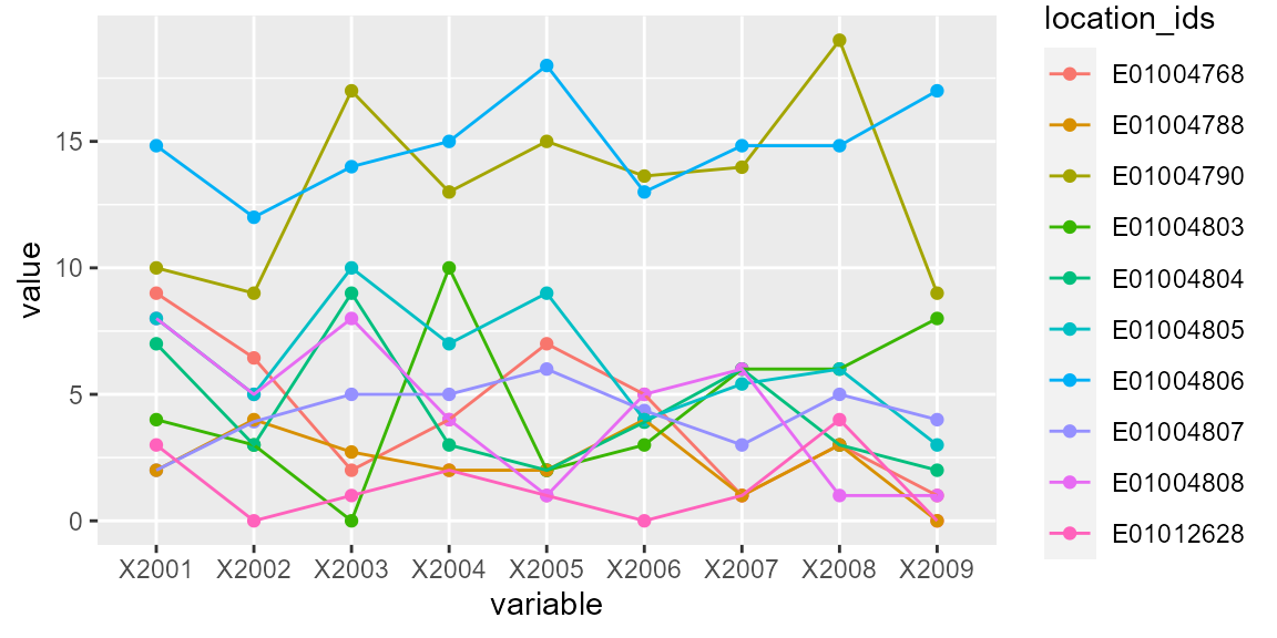

Figure 3: Replacing outliers with mean observation

Setting replace_with = 2, that is to replace the outlier points with the ‘mean of the row observations’, the function generates outputs re-plotted in Figure 3.

(vii) ‘Other’ functions

Please see the akmedoids user manual for the remaining data manipulation functions.

2. Data Clustering

Table 2 shows the two main functions required to carry out the longitudinal clustering and generate the descriptive statistics of the resulting groups. The relevant functions are akclustr and print_akstats. The akclustr function clusters trajectories according to the similarities of their long-term trends, while the print_akstats function extracts descriptive and change statistics for each of the clusters. The former also generates quality plots for the best cluster solution.

The long-term trends of trajectories are defined in terms of a set of OLS regression lines. This allows the clustering function to classify the final groupings in terms of their slopes as rising, stable, and falling. The key benefits of this implementation is that it allows the clustering process to ignore the short-term fluctuations of actual trajectories and focus on their long-term linear trends. Adepeju and colleagues (2021) applied this technique in crime concentration research for measuring long-term inequalities in the exposure to crime at find-grained spatial scales.

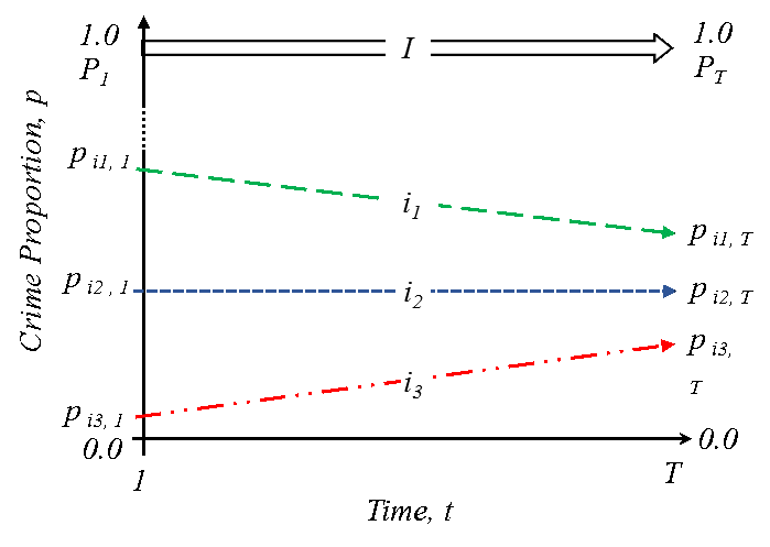
Figure 4: Long-time linear trends of relative (proportion, p) crime exposure. Three inequality trends: trajectory i1: crime exposure is falling faster, i2, crime exposure is falling at the same rate, and i3, crime exposure is falling slower or increasing, relatively to the citywide trend. (Source: Adepeju et al. 2021)

Their implementation was informed by the conceptual (inequality) framework shown in Figure 4. That said, akmedoids can be deployed on any measure (counts, rates) and is not limited to criminology, but rather, any field where the aim is to cluster longitudinal data based on long-term trajectories. By mapping the resulting trend lines grouping to the original trajectories, various performance statistics can be generated.

In addition to the use of trend lines, the akmedoids makes two other modifications to the expectation-maximisation clustering routines (Celeux and Govaert 1992). First, the akmedoids implements an anchored median-based initialisation strategy for the clustering to begin. The purpose behind this step is to give the algorithm a theoretically-driven starting point and try and ensure that heterogenous trend slopes end up in different clusters (Khan and Ahmad (2004); Steinley and Brusco (2007)). Second, instead of recomputing centroids based on the mean distances between each trajectory trend lines and the cluster centers, the median of each cluster is selected and then used as the next centroid. This then becomes the new anchor for the current iteration of the expectation-maximisation step (Celeux and Govaert 1992). This strategy is implemented in order to minimize the impact of outliers. The iteration then continues until an objective function is maximised.

Table 2. Data clustering functions

SN	Function	Title	Description
1	akclustr	Anchored k-medoids clustering	Clusters trajectories into a k number of groups according to the similarities in their long-term trend and determines the best solution based on the Silhouette width measure or the Calinski-Harabasz criterion
2	print_akstats	Descriptive (Change) statistics of clusters	Generates the descriptive and change statistics of groups, and also plots the groups performances
3	plot_akstats	Plots of cluster groups	Generates different plots of cluster groups

#Visualizing the proportion data

#view the first few rows
head(prop_crime_per200_people)
#>   location_ids X2001 X2002 X2003 X2004 X2005 X2006 X2007 X2008 X2009
#> 1    E01012628  0.10  0.13  0.04  0.09  0.21  0.19  0.05  0.14  0.17
#> 2    E01004768  0.12  0.28  0.13  0.09  0.09  0.17  0.04  0.08  0.00
#> 3    E01004803  0.08  0.11  0.16  0.13  0.17  0.16  0.17  0.15  0.17
#> 4    E01004804  0.07  0.07  0.00  0.18  0.04  0.06  0.12  0.08  0.24
#> 5    E01004807  0.15  0.08  0.18  0.06  0.04  0.08  0.12  0.04  0.06
#> 6    E01004808  0.11  0.11  0.18  0.14  0.22  0.11  0.16  0.13  0.16

#prop_crime_per200_people_melt <- melt(prop_crime_per200_people, id="location_ids") 
coln <- colnames(prop_crime_per200_people)[2:length(colnames(prop_crime_per200_people))]
code_ <- rep(prop_crime_per200_people$location_ids, ncol(prop_crime_per200_people)-1)
d_bind <- NULL
  for(v in seq_len(ncol(prop_crime_per200_people)-1)){
    d_bind <- c(d_bind, prop_crime_per200_people[,(v+1)])
  }

prop_crime_per200_people_melt <- data.frame(cbind(location_ids=as.character(code_), variable =
                        rep(coln,
                        each=length(prop_crime_per200_people$location_ids)), value=d_bind))

#plot function
#options(rgl.useNULL = TRUE)
p <-  ggplot(prop_crime_per200_people_melt, aes(x=variable, y=value,
            group=location_ids, color=location_ids)) + 
            geom_point() + 
            geom_line()

#options(rgl.useNULL = TRUE)
print(p)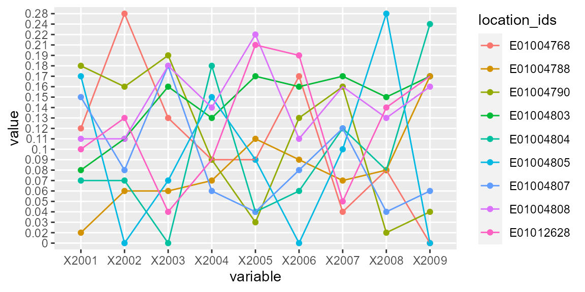

Figure 5: Trajectory of crime proportions over time

In the following sections, we provide a worked example of clustering with akclustr function using the prop_crime_per200_people object. The function will generate cluster solution over a set of k values, determine the optimal value of k. The print_akstats function will then be applied to generate the descriptive summary and the change statistics of the clusters. The prop_crime_per200_people object is plotted in 5.

(i) akclustr function

Dataset:

Each trajectory in Figure 5 represents the proportion of crimes per 200 residents in each location over time. The goal is to first extract the inequality trend lines such as in Figure 4 and then cluster them according to the similarity of their slopes. For the akclustr function, a user sets the k value which may be an integer or a vector of length two specifying the minimum and maximum numbers of clusters to loop through. In the latter case, the akclustr function employs either the Silhouette (Rousseeuw (1987))) or the Calinski_Harabasz score (Caliński and Harabasz (1974); Genolini and Falissard (2010)) to determine the best cluster solution. In other words, it determines the k value that optimizes the specified criterion. The verbose argument can be used to control the processing messages. The function is executed as follows:

#clustering
akObj <- akclustr(prop_crime_per200_people, id_field = TRUE, 
                                method = "linear", k = c(3,8), crit = "Calinski_Harabasz", verbose=TRUE)
#> [1] "Processing...."
#> [1] ".............."
#> [1] "solution of k = 3 determined!"
#> [1] "solution of k = 4 determined!"
#> [1] "solution of k = 5 determined!"
#> [1] "solution of k = 6 determined!"
#> [1] "solution of k = 7 determined!"
#> [1] "solution of k = 8 determined!"

In order to preview all the variables of the quality_plot object, type:

names(akObj)
#> [1] "traj"             "id_field"         "solutions"        "qualitycriterion"
#> [5] "optimal_k"        "qualityCrit.List" "qltyplot"

• The description of these variables are as follow:

  • traj - returns the input data set used for the clustering.

  • id_field - indicates whether the input data set included the id field.

  • solutions - the list of cluster solutions by k values.

  • qualitycriterion - the quality criterion specified.

  • optimal_k - the optimal value of k as determined by the quality criterion.

  • qualityCrit.List - the estimated quality of cluster solutions by k values.

  • qltyplot - the plot of qualityCrit.List, with a red vertical line to indicate the optimal value of k.

Accessing the optimal solution*

The qualityCrit.List can be viewed graphically by setting the quality_plot argument as TRUE. Also, the plot may still be accessed after clustering by printing the variable akObj$qltyplot.

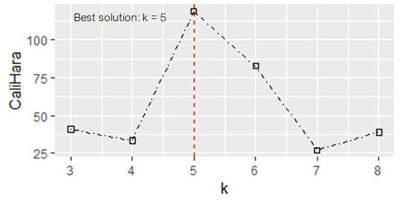
Figure 6: Clustering performance at different values of k

From (Figure 6), the best value of k is the highest at k=5, and therefore determined as the best solution. It is recommended that the determination based on either of the quality criteria should be used complementarily with users judgment in relation to the problem at hand.

Given a value of k, the group membership (labels) of its cluster solution can be extracted by entering k'= k - 2) into the variable akObj$solutions[[k']]. E.g.

#5-group clusters
akObj$solutions[[3]] #for `k=5` solution
#> [1] "D" "A" "D" "E" "B" "C" "E" "A" "C"
#> attr(,"cluster labels for k =")
#> [1] 5

Also, note that the indexes of the group memberships correspond to that of the trajectory object (prop_crime_per200_people) inputted into the function. That is, the membership labels, "D", "A", "A", .... are the group membership of the trajectories "E01012628","E01004768","E01004803",... of the object prop_crime_per200_people.

(ii) print_akstats function:

The properties (i.e. the descriptive and change statistics) of a cluster solutions (i.e. solution for any value of k) such as in k = 5 above can be generated by using the special print function print_akstats. The print function takes as input the akobject class, e.g. akObj. The descriptive statistics shows the group memberships and their performances in terms of their shares of the proportion measure captured over time. The change statistics shows the information regarding the direction variances of the groups in relation to reference direction. In trajectory clustering analysis, the resulting groups are often re-classified into larger classes based on the slopes, such as Decreasing, Stable, or Increasing classes (Weisburd et al. (2004); Andresen et al. 2017). The slope of a group is the angle made by the medoid of the group relative to a reference line (\(R\)). The reference argument is specified as 1, 2 or 3, representing the mean trajectory, medoid trajectory, or a horizontal line with slope = 0, respectively. Let \(\vartheta_{1}\) and \(\vartheta_{n}\) represent the angular deviations of the group medoids with the lowest slope (negative) and highest (positive) slopes, respectively.

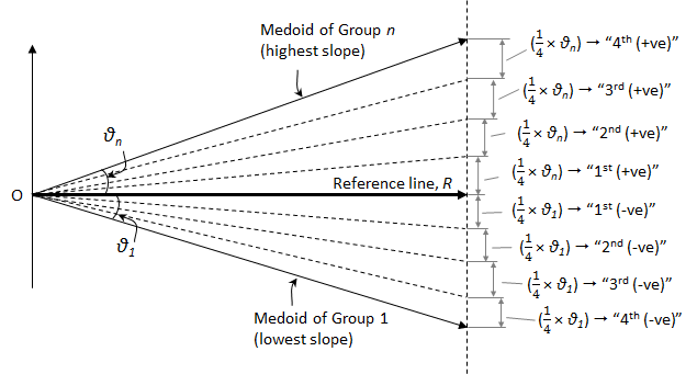
Figure 7: Quantile sub-divisions of most-diverging groups (n_quant=4)

If we sub-divide each of these slopes into a specified number of equal intervals (quantiles), the specific interval within which each group medoid falls can be determined. This specification is made using the n_quant argument. Figure 7 illustrates the quantiles sub-divisions for n_quant = 4.

In addition to the slope composition of trajectories found in each group, the quantile location of each group medoid can be used to further categorize the groups into larger classes. We refer users to the package user manual for more details about these parameters. Using the current example, the function can be ran as follows:

#Specifying the optimal solution, output$optimal_k (i.e. `k = 5`) and using `stacked` type graph
prpties = print_akstats(akObj, k = 5, show_plots = FALSE)
#> Warning: `fun.y` is deprecated. Use `fun` instead.

prpties
#> $descriptive_stats
#>   group n n(%) %Prop.time1 %Prop.timeT Change %Change
#> 1     A 2 22.2          30           4    -26    -650
#> 2     B 1 11.1          15         5.9   -9.1  -154.2
#> 3     C 2 22.2          28        15.8  -12.2   -77.2
#> 4     D 2 22.2          18        33.7   15.7    46.6
#> 5     E 2 22.2           9        40.6   31.6    77.8
#> 
#> $change_stats
#>   group sn %+ve Traj. %-ve Traj. Qtl:1st-4th
#> 1     A  1          0        100   4th (-ve)
#> 2     B  2          0        100   3rd (-ve)
#> 3     C  3        100          0   1st (+ve)
#> 4     D  4        100          0   3rd (+ve)
#> 5     E  5        100          0   4th (+ve)

(iii) plot_akstats function:

The above printouts represent the properties (i.e. the descriptive and change properties) of the clusters. Note: the show_plots argument of print_akstats function, if set as TRUE, will produce the plot of group trajectories, representing the group directional change over time. However, the plot_akstats has been designed to generate different performance plots of the groups. See below:

1. Group trajectories (directional change over time)

  #options(rgl.useNULL = TRUE)
  plot_akstats(akObj, k = 5, type="lines", y_scaling="fixed")
#> Warning: `fun.y` is deprecated. Use `fun` instead.
#> $cluster_plot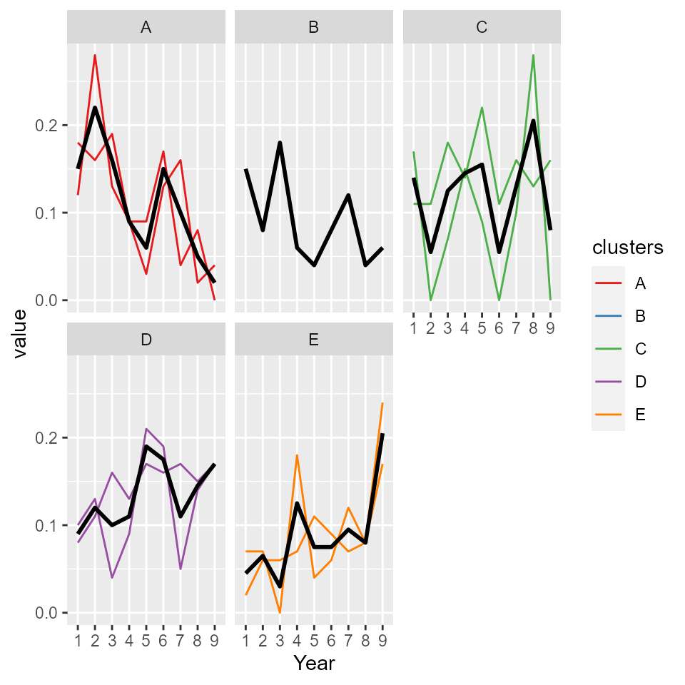

2. Proportional change of groups change over time

  #options(rgl.useNULL = TRUE)
  plot_akstats(akObj, k = 5, reference = 1, n_quant = 4, type="stacked")
#> $cluster_plot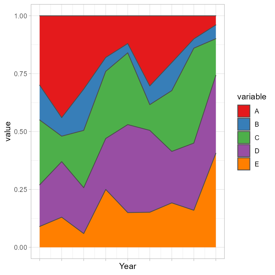

In the context of the long-term inequality study, broad conclusions can be made from both the statistical properties and the plots regarding relative crime exposure in the area represented by each group or class (Adepeju et al. 2021). For example, whilst relative crime exposure have declined in 33.3% (groups A and B) of the study area, the relative crime exposure have risen in 44.4% (groups D and E) of the area. The relative crime exposure can be said to be stable in 22.2% (group C) of the area, based on its close proximity to the reference line. The medoid of the group falls within the \(1^{st}(+ve)\) quantile (see Figure ). In essence, we determine that groups A and B belong to the Decreasing class, while groups D and E belong to the Increasing class.

It is important to state that this proposed classification method is simply advisory; you may devise a different approach or interpretation depending on your research questions and data.

By changing the argument type="lines" to type="stacked", a quality plot is generated instead (see Figure ). Note that these plots make use of functions within the ggplot2 library (Wickham 2016). For a more customized visualization, we recommend that users deploy the ggplot2 library directly.

Table 3. field description of clustering outputs

SN	field	Description
1	group	group membershp
2	n	size (no.of.trajectories.)
3	n(%)	% size
4	%Prop.time1	% proportion of obs. at time 1 (2001)
5	%Prop.timeT	proportion of obs. at time T (2009)
6	Change	absolute change in proportion between time1 and timeT
7	%Change	% change in proportion between time 1 and time T
8	%+ve Traj.	% of trajectories with positive slopes
9	%-ve Traj.	% of trajectories with negative slopes
10	Qtl:1st-4th	Position of a group medoid in the quantile subdivisions

Conclusion

The akmedoids package has been developed in order to aid the replication of a place-based crime inequality investigation conducted in Adepeju, Langton, and Bannister (2021). Meanwhile, the utility of the functions in this package are not limited to criminology, but rather can be applicable to longitudinal datasets more generally. This package is being updated on a regular basis to add more functionalities to the existing functions and add new functions to carry out other longitudinal data analysis.

We encourage users to report any bugs encountered while using the package so that they can be fixed immediately. Welcome contributions to this package which will be acknowledged accordingly.

References

Adepeju, M., S. Langton, and J. Bannister. 2021. “Anchored K-Medoids: A Novel Adaptation of K-Medoids Further Refined to Measure Inequality in the Exposure to Crime Across Micro Places.” Journal of Computational Social Science. https://doi.org/10.1007/s42001-021-00103-1.

Caliński, T., and J. Harabasz. 1974. “A Dendrite Method for Cluster Analysis.” Communications in Statistics-Theory and Methods 3(1): 1–27.

Celeux, G., and G. Govaert. 1992. “A Classification Em Algorithm for Clustering and Two Stochastic Versions.” Computational Statistics 14(3): 315–32.

Genolini, C., and B. Falissard. 2010. “Kml and Kml3d: R Packages to Cluster Longitudinal Data.” Computational Statistics 25(2): 317–28.

Griffith, E., and J. M. Chavez. 2004. “Communities, Street Guns and Homicide Trajectories in Chicago, 1980–1995: Merging Methods for Examining Homicide Trends Across Space and Time.” Criminology 42(4): 941–78.

Khan, S. S, and A. Ahmad. 2004. “Cluster Center Initialization Algorithm for K-Means Clustering.” Pattern Recognition Letters 25(11): 1293–1302.

Rousseeuw, P. J. 1987. “Silhouettes: A Graphical Aid to the Interpretation and Validation of Cluster Analysis.” Journal of Computational and Applied Mathematics, no. 20: 53–65.

Steinley, D., and M. J. Brusco. 2007. “Initializing K-Means Batch Clustering: A Critical Evaluation of Several Techniques.” Journal of Classification 24(1): 99–121.

Weisburd, D., S. Lum, C. Lum, and S. M. Lum. 2004. “Trajectories of Crime at Places: A Longitudinal Study of Street Segments in the City of Seattle.” Criminology 42(2): 283–322.

Wickham, H. 2016. Elegant Graphics for Data Analysis. Spring-Verlag New York.