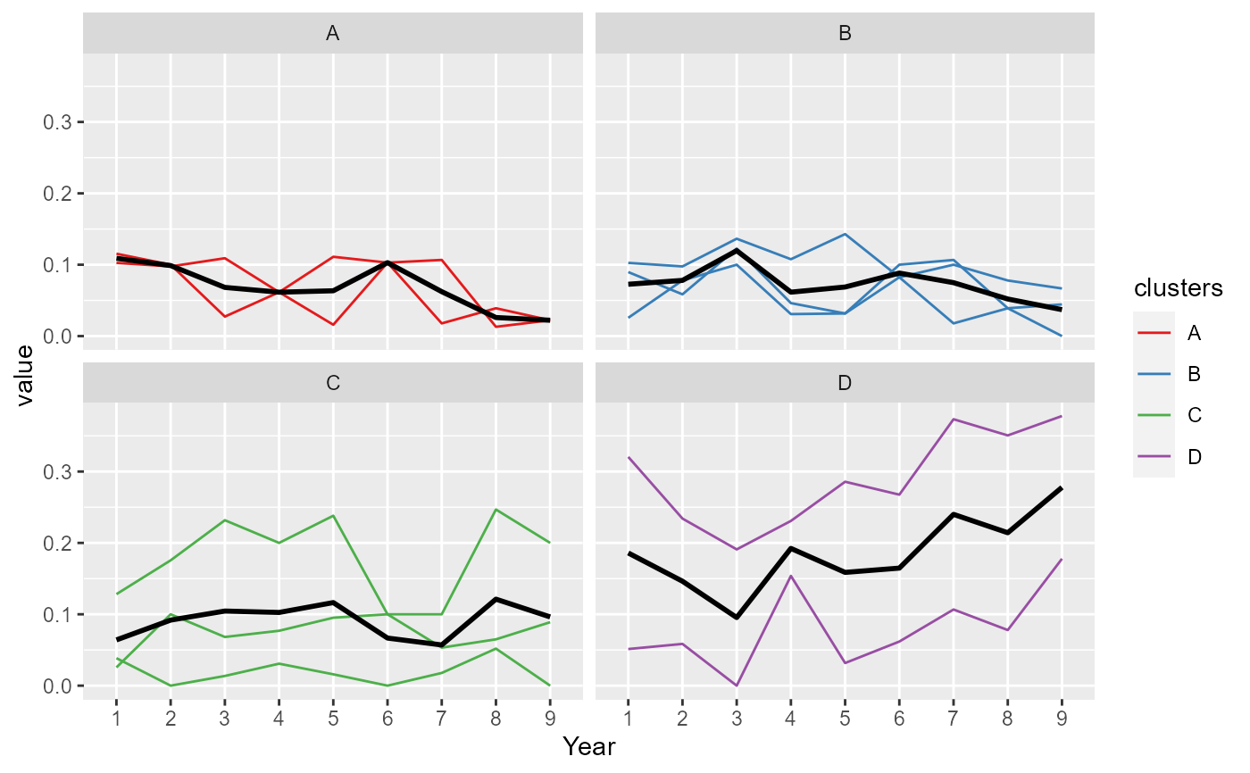
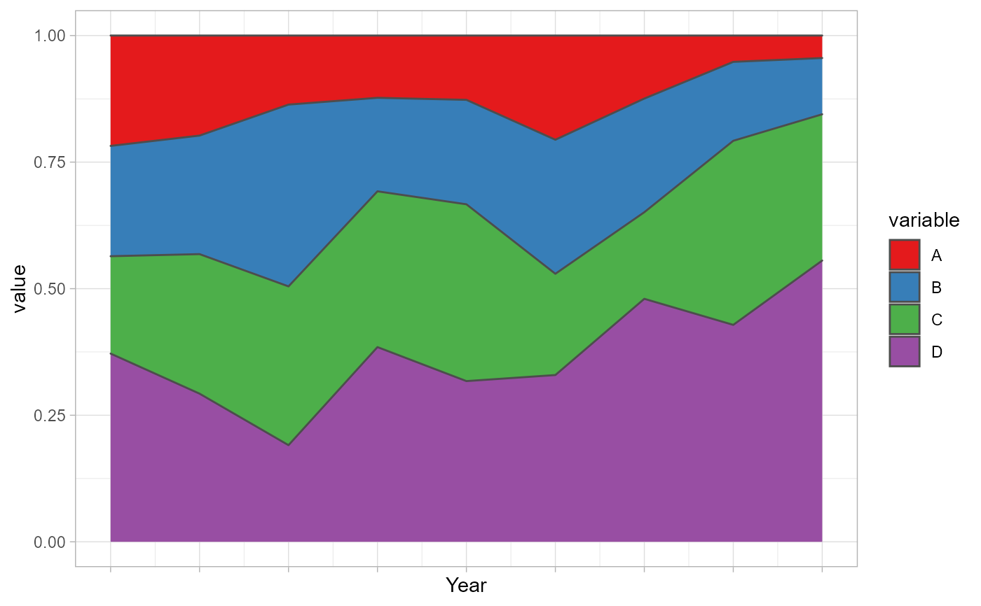
Plot of cluster groups. — plot_akstats • akmedoids

Takes the 'ak_object' from the 'akclustr' as input and produce either the 'line' plot or 'stacked' histogram.

plot_akstats(
  ak_object,
  k = 3,
  reference = 1,
  n_quant = 4,
  type = "lines",
  y_scaling = "fixed"
)

Arguments

ak_object	An output of `akclustr` function. The object contains individual trajectories and their cluster solution(s) at the specified values of `k`. Also, includes the optimal value of `k` based on the criterion specified. at (different) values of `k` the `traj`.
k	[integer] `k` cluster to generate its solution.
reference	[numeric] Specifying the reference line from which the direction of each group is measured. Options are: `1`: slope of mean trajectory, `2`: slope of medoid trajectory, `3`: slope of a horizontal line (i.e. slope = 0). Default: `1`.
n_quant	[numeric] Number of equal intervals (quantiles) to create between the reference line `(R)` and the medoids `(M)` of the most-diverging groups of both sides of `(R)`. Default is `4` - meaning quartile subdivisions on each side of `(R)`. In this scenario, the function returns the quartile in which the medoid of each group falls. This result can be used to further categorize the groups into 'classes'. For example, groups that fall within the `1st` quartile may be classified as 'Stable' groups (Adepeju et al. 2021).
type	[character] plot type. Available options are: `"lines"` and `"stacked"`.
y_scaling	[character] works only if `type="lines"`. `y_scaling` set the vertical scales of the cluster panels. Options are: `"fixed"`: uses uniform scale for all panels, `"free"`: uses variable scales for panels.

Value

A plot showing group membership or sizes (proportion) and statistics.

Details

Generates the plots of cluster groups - same plots generated by the 'show_plots' argument of print_akstats. The function draw from the functionalities of the ggplot2 library. For a more customized visualisation, we recommend that users deploy ggplot2 directly (Wickham H. (2016)).

References

1. Adepeju, M. et al. (2021). Anchored k-medoids: A novel adaptation of k-medoids further refined to measure inequality in the exposure to crime across micro places, doi: 10.1007/s42001-021-00103-1.

2. Wickham H. (2016). Elegant graphics for Data Analysis. Spring-Verlag New York (2016).

Examples


data(traj)

trajectry <- data_imputation(traj, id_field = TRUE, method = 1,
replace_with = 1, fill_zeros = FALSE)
#> [1] "8 entries were found/filled!"

print(trajectry$CompleteData)
#>    location_ids X2001  X2002     X2003 X2004 X2005     X2006  X2007 X2008 X2009
#> 1     E01012628     3  0.000  1.000000     2     1  0.000000  1.000     4     0
#> 2     E01004768     9  5.125  2.000000     4     7  5.000000  1.000     3     1
#> 3     E01004803     4  3.000  0.000000    10     2  3.000000  6.000     6     8
#> 4     E01004804     7  3.000  9.000000     3     2  4.857143  6.000     3     2
#> 5     E01004807     2  5.125  5.000000     5     6  4.857143  3.000     5     4
#> 6     E01004808     8  5.000  8.000000     4     1  5.000000  6.000     1     1
#> 7     E01004788     2  4.000  7.333333     2     2  4.000000  1.000     3     0
#> 8     E01004790    10  9.000 17.000000    13    15  4.857143  5.625    19     9
#> 9     E01004805     8  5.000 10.000000     7     9  4.000000  5.625     6     3
#> 10    E01004806    25 12.000 14.000000    15    18 13.000000 21.000    27    17

trajectry <- props(trajectry$CompleteData, id_field = TRUE)

aksolution <- akclustr(trajectry, id_field = TRUE,
method = "linear", k = c(3,5), crit='Calinski_Harabasz')
#> [1] "Processing...."
#> [1] ".............."
#> [1] "solution of k = 3 determined!"
#> [1] "solution of k = 4 determined!"
#> [1] "solution of k = 5 determined!"

plot_akstats(aksolution, k = 4, type="lines",
y_scaling="fixed")
#> Warning: `fun.y` is deprecated. Use `fun` instead.
#> $cluster_plot
#> 

plot_akstats(aksolution, k = 4, reference = 1,
n_quant = 4, type="stacked")
#> $cluster_plot
#>